本系列连载文章:
- 七天搞定SAS(七):常用统计模型
- 七天搞定SAS(六):宏的编写、程序调错
- 七天搞定SAS(五):数据操作与合并
- 七天搞定SAS(四):数据输出
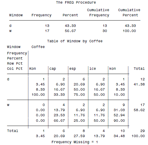
- 七天搞定SAS(三):基本模块调用(格式、计数、概要统计、排序等)
- 七天搞定SAS(二):基本操作(判断、运算、基本函数)
- 七天搞定SAS(一):数据的导入、数据结构
其实最后一天,反而是任务最繁重的。这一天,需要纵览SAS的各个常用的统计模块。BTW,在用惯了ggplot2之后,再也不认为有任何理由用其他软件画图了...所以SAS的图形模块自动被我无视(貌似很多SAS用户也一直在吐槽这东西着实不好使)。
SAS里面的概要统计:PROC MEANS
其实前几天也说过了PROC MEANS,不过这里稍稍补充一点置信区间的东西吧。其实它的参数真的挺多的:
- CLM:双侧置信区间
- CSS:调整平方和
- CV:变异系数
- KURTOSIS:峰度
- LCLM :单侧置信区间——左侧
- MAX:最大值
- MEAN:均值
- MIN:最小值
- MODE:众数
- N :非缺失值个数
- NMISS:缺失值个数
- MEDIAN(P50):中位数
- RANGE:范围
- SKEWNESS:偏度
- STDDEV:标准差
- STDERR:均值的标准误
- SUM:求和
- SUMWGT:加权求和
- UCLM:单侧置信区间:右侧
- USS:未修正的平方和
- VAR:方差
ode variance
- PROBT:t统计量对应的p值
- T:t统计量
- Q3 (P75):75%分位数,etc.
- P10:10%分位数,etc.
在调用CLM的时候需要指定ALPHA:
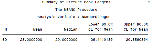
DATA booklengths;
INFILE 'c:\MyRawData\Picbooks.dat';
INPUT NumberOfPages @@;
RUN;
*Produce summary statistics;
PROC MEANS DATA=booklengths N MEAN MEDIAN CLM ALPHA=.10;
TITLE 'Summary of Picture Book Lengths';
RUN;
结果如下:
SAS里面的相关性分析:PROC CORR
虽然correlation一直被各种批判,但是往往在拿到数据的第一步、毫无idea的时候,correlation还是值得一看的参考指标。SAS里面的PROC CORR提供了相应的功能。
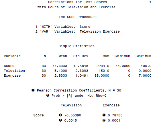
PROC CORR DATA = class;
VAR Television Exercise;
WITH Score;
TITLE ’Correlations for Test Scores’;
TITLE2 ’With Hours of Television and Exercise’;
RUN;
SAS的相关性分析结果输出如下:
SAS里面的基本回归分析:PROC REG
类似于R中的lm(),这个实在是没什么好说的了,最基本的最小二乘法。
DATA hits;
INFILE 'c:\MyRawData\Baseball.dat';
INPUT Height Distance @@;
RUN;
* Perform regression analysis;
PROC REG DATA = hits;
MODEL Distance = Height;
TITLE 'Results of Regression Analysis';
RUN;
SAS的输出结果如下: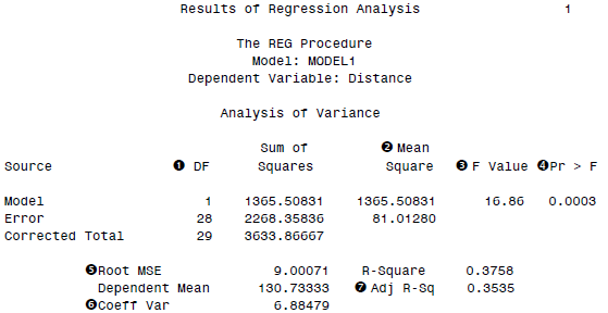
包含了回归模型的基本统计量。我们一般更关注的回归系数:
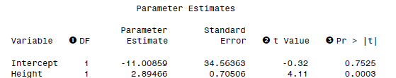
到这里,我的感慨就是:真的很像Stata呀!值得注意的是,REG有很多可选的参数,对于这些参数是干嘛用的,最权威的自然还是SAS官方的文档:http://support.sas.com/documentation/cdl/en/statug/63033/HTML/default/viewer.htm#statug_reg_sect007.htm。其实熟悉了SAS的语法和工作模式之后,具体到某个模型还是看官方文档比较舒服。不愧是商业软件啊,文档写的都很专业,有很多模型选择问题其实看看文档就能多少明白一些了。
比如PROC REG的参数就有:
| Option | Description |
|---|---|
| Data Set Options | |
| DATA= | names a data set to use for the regression |
| OUTEST= | outputs a data set that contains parameter estimates and other model fit summary statistics |
| OUTSSCP= | outputs a data set that contains sums of squares and crossproducts |
| COVOUT | outputs the covariance matrix for parameter estimates to the OUTEST= data set |
| EDF | outputs the number of regressors, the error degrees of freedom, and the model  to the OUTEST= data set to the OUTEST= data set |
| OUTSEB | outputs standard errors of the parameter estimates to the OUTEST= data set |
| OUTSTB | outputs standardized parameter estimates to the OUTEST= data set. Use only with the RIDGE= or PCOMIT= option. |
| OUTVIF | outputs the variance inflation factors to the OUTEST= data set. Use only with the RIDGE= or PCOMIT= option. |
| PCOMIT= | performs incomplete principal component analysis and outputs estimates to the OUTEST= data set |
| PRESS | outputs the PRESS statistic to the OUTEST= data set |
| RIDGE= | performs ridge regression analysis and outputs estimates to the OUTEST= data set |
| RSQUARE | same effect as the EDF option |
| TABLEOUT | outputs standard errors, confidence limits, and associated test statistics of the parameter estimates to the OUTEST= data set |
| ODS Graphics Options | |
| PLOTS= | produces ODS graphical displays |
| Traditional Graphics Options | |
| ANNOTATE= | specifies an annotation data set |
| GOUT= | specifies the graphics catalog in which graphics output is saved |
| Display Options | |
| CORR | displays correlation matrix for variables listed in MODEL and VAR statements |
| SIMPLE | displays simple statistics for each variable listed in MODEL and VAR statements |
| USCCP | displays uncorrected sums of squares and crossproducts matrix |
| ALL | displays all statistics (CORR, SIMPLE, and USSCP) |
| NOPRINT | suppresses output |
| LINEPRINTER | creates plots requested as line printer plot |
| Other Options | |
| ALPHA= | sets significance value for confidence and prediction intervals and tests |
| SINGULAR= | sets criterion for checking for singularity |
SAS里面的基本方差分析:PROC ANOVA
方差分析也就不赘述了,其实我感觉没有回归分析更用的普遍...这俩东西某种程度上也是一回事儿,看怎么理解了。
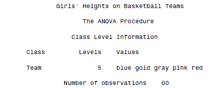
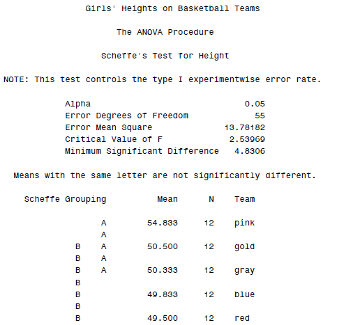
PROC ANOVA DATA = basket;
CLASS Team;
MODEL Height = Team;
MEANS Team / SCHEFFE;
TITLE ”Girls’ Heights on Basketball Teams”;
RUN;
SAS的输出如下:
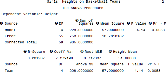
先是用作分类的变量的基本统计。然后是模型的基本统计:
最后是各个组的分析结果(两两比较,由于指定了SCHEFFE参数):
SAS中的离散被解释变量模型:PROC LOGISTIC和PROC GENMOD
最简单的离散被解释变量模型就是logit了,在SAS里面有直接的PROC LOGISTIC。官方文档在此:http://support.sas.com/documentation/cdl/en/statug/63033/HTML/default/viewer.htm#logistic_toc.htm
语法自然是一如既往的简单:
proc logistic;
model y=x1 x2;
run;
结果返回:
| Model Information | |
|---|---|
| Data Set | WORK.INGOTS |
| Response Variable (Events) | r |
| Response Variable (Trials) | n |
| Model | binary logit |
| Optimization Technique | Fisher's scoring |
| Number of Observations Read | 19 |
|---|---|
| Number of Observations Used | 19 |
| Sum of Frequencies Read | 387 |
| Sum of Frequencies Used | 387 |
首先自然是模型的统计信息。然后是数据的统计:
| Response Profile | ||
|---|---|---|
| Ordered Value |
Binary Outcome | Total Frequency |
| 1 | Event | 12 |
| 2 | Nonevent | 375 |
| Model Convergence Status |
|---|
| Convergence criterion (GCONV=1E-8) satisfied |
然后是假设检验:
| Model Fit Statistics | ||
|---|---|---|
| Criterion | Intercept Only |
Intercept and Covariates |
| AIC | 108.988 | 103.222 |
| SC | 112.947 | 119.056 |
| -2 Log L | 106.988 | 95.222 |
| Testing Global Null Hypothesis: BETA=0 | |||
|---|---|---|---|
| Test | Chi-Square | DF | Pr > ChiSq |
| Likelihood Ratio | 11.7663 | 3 | 0.0082 |
| Score | 16.5417 | 3 | 0.0009 |
| Wald | 13.4588 | 3 | 0.0037 |
最后是参数估计:
| Analysis of Maximum Likelihood Estimates | |||||
|---|---|---|---|---|---|
| Parameter | DF | Estimate | Standard Error |
Wald Chi-Square |
Pr > ChiSq |
| Intercept | 1 | -5.9901 | 1.6666 | 12.9182 | 0.0003 |
| Heat | 1 | 0.0963 | 0.0471 | 4.1895 | 0.0407 |
| Soak | 1 | 0.2996 | 0.7551 | 0.1574 | 0.6916 |
| Heat*Soak | 1 | -0.00884 | 0.0253 | 0.1219 | 0.7270 |
而对于泊松模型,则需要PROC GENMOD。我觉得我一一个列出这些模型已经超出了这篇笔记的范围了...所以干脆就改成简单翻译一下各个PROC的主要模型吧。说过了,学习模型不是主要的目的——模型终究不该通过软件来学...虽然SAS的user guide真的还算是比较好的统计学教材呢。
SAS里面的PROC一览
除了上面说到的PROC,SAS当然还有更多强大的模块。我就顺手一一点开看看这些东西都能做什么...
- The ACECLUS Procedure:聚类的协方差矩阵近似估计(approximate covariance estimation for clustering)
- The ANOVA Procedure:方差分析
- The BOXPLOT Procedure:箱形图
- The CALIS Procedure:结构方程模型
- The CANCORR Procedure:典型相关分析
- The CANDISC Procedure:主成分分析和典型相关分析
- The CATMOD Procedure:类别分析
- The CLUSTER Procedure:聚类分析,包括11种(average linkage, the centroid method, complete linkage, density linkage (including Wong’s hybrid and th-nearest-neighbor methods), maximum likelihood for mixtures of spherical multivariate normal distributions with equal variances but possibly unequal mixing proportions, the flexible-beta method, McQuitty’s similarity analysis, the median method, single linkage, two-stage density linkage, and Ward’s minimum-variance method,机器翻译为:平均联动,重心法,完全连锁,密度连接(包括Wong混合模型,最近邻的方法),最大的可能性,McQuitty的相似性分析,中位数法,单联动,两阶段密度联动,Ward最小方差法)。
- The CORRESP Procedure:简单的对应分析和多元对应分析(MCA)
- The DISCRIM Procedure:生成分类器的判别标准
- The DISTANCE Procedure:距离,不相似或相似性分析
- The FACTOR Procedure:因子分析和因子旋转
- The FASTCLUS Procedure:快速聚类分析(给定计算出来的距离)
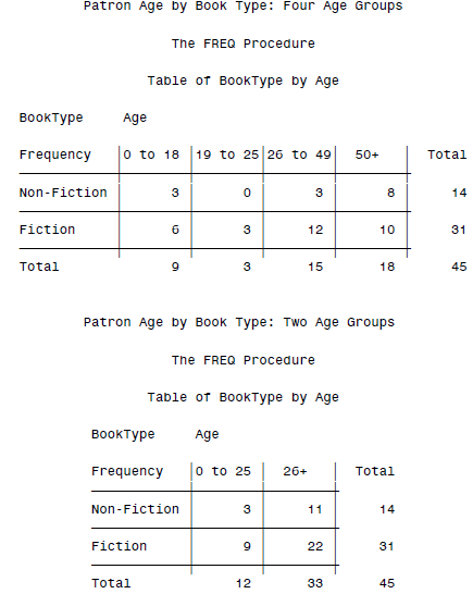
- The FREQ Procedure:频率统计
- The GAM Procedure:广义可加模型
- The GENMOD Procedure:广义线性模型,泊松回归、贝叶斯回归等
- The GLIMMIX Procedure: generalized linear mixed models (GLMM),广义线性混合模型
- The GLM Procedure:最小二乘法模型,包括回归、方差分析、协方差分析、多元方差分析、偏相关。
- The GLMMOD Procedure:广义线性模型设计
- The GLMPOWER Procedure:预测力和样本大小的线性模型分析
- The GLMSELECT Procedure:变量选择,包括Lasso和LAR等。
- The HPMIXED Procedure:线性混合模型,包括固定效应、随机效应等。
- The INBREED Procedure:协方差或近亲繁殖系数。
- The KDE Procedure:单变量和二元核密度估计
- The KRIGE2D Procedure:二维克里格法,包括各向异性和嵌套的半方差图模型
- The LATTICE Procedure:简单的栅格设计实验的方差分析和协方差分析
- The LIFEREG Procedure:生存分析中的参数模型,包括各种截尾数据
- The LIFETEST Procedure:生存分析的相关检验
- The LOESS Procedure:非参数模型、多维数据、支持多因变量、直接和插值的kd树、统计推断、自动平滑参数的选择、执行迭代时有异常值的数据。
- The LOGISTIC Procedure:logit回归
- The MCMC Procedure:Markov chain Monte Carlo (MCMC) simulation-马尔可夫链蒙特卡洛模拟
- The MDS Procedure:Multidimensional scaling (MDS)-多维标度模型
- The MI Procedure:缺失值处理
- The MIANALYZE Procedure:缺失值分析
- The MIXED Procedure:混合线性模型,面板数据的常用模型
- The MODECLUS Procedure:各种参数、非参数的聚类模型
- The MULTTEST Procedure:多重检验的p值调整
- The NESTED Procedure:嵌套的随机效应模型(nested random effects model)
- The NLIN Procedure:非线性回归模型
- The NLMIXED Procedure:非线性混合模型(固定效应和随机效应都是非线性的)
- The NPAR1WAY Procedure:位置和规模差异的非参数检验
- The ORTHOREG Procedure:更精准的广义线性模型(Gentleman-Givens 变换来求解QR分解)
- The PHREG Procedure: Cox proportional hazards model-Cox比例风险模型
- The PLAN Procedure:因子实验设计
- The PLS Procedure:partial least squares (PLS)-偏最小二乘法
- The POWER Procedure:模型能力和样本量分析
- The Power and Sample Size Application:桌面版的能力和样本量分析程序
- The PRINCOMP Procedure:主成份分析
- The PRINQUAL Procedure:定质,定量,或混合数据的主成分分析(PCA)
- The PROBIT Procedure:probit回归
- The QUANTREG Procedure:分位数回归
- The REG Procedure:最小二乘回归
- The ROBUSTREG Procedure:稳健回归(剔除离群点影响)
- The RSREG Procedure:二次响应回归模型
- The SCORE Procedure:打分
- The SEQDESIGN Procedure:临床试验的中期设计
- The SEQTEST Procedure:临床试验的中期分析
- The SIM2D Procedure:高斯随机场的空间模拟(anisotropic and nested semivariogram models)
- The SIMNORMAL Procedure:生成高斯分布的模拟数据
- The STDIZE Procedure:标准化数据
- The STEPDISC Procedure:逐步回归(变量选择)
- The SURVEYFREQ Procedure:单向或者多向频率和交叉表的抽样调查数据分析
- The SURVEYLOGISTIC Procedure:抽样调查的logit回归
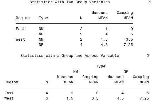
- The SURVEYMEANS Procedure:抽样调查数据的概要统计
- The SURVEYREG Procedure:抽样调查数据的回归分析
- The SURVEYSELECT Procedure:选择基于概率的随机样本
- The TCALIS Procedure:结构方程模型(目测是CALIS的加强版)
- The TPSPLINE Procedure:补偿最小二乘法来拟合非参数回归模型
- The TRANSREG Procedure:transformation regression(一系列基于最小二乘法的变换)
- The TREE Procedure:树状图
- The TTEST Procedure:各种情况下的t检验
- The VARCLUS Procedure:不相交或分层聚类
- The VARCOMP Procedure:含有随机效应的广义线性模型
- The VARIOGRAM Procedure:二维空间数据的连续性分析